44 how to change axis labels in excel 2013

Use defined names to automatically update a chart range - Office Select cells A1:B4. On the Insert tab, click a chart, and then click a chart type. Click the Design tab, click the Select Data in the Data group. Under Legend Entries (Series), click Edit. In the Series values box, type =Sheet1!Sales, and then click OK. Under Horizontal (Category) Axis Labels, click Edit. [Solved] : How to Fix MS Excel Crash Issue Restart Excel in normal mode and go to File> Options> Add-ins Choose COM Add-ins from the drop-down and click Go Uncheck all the checkboxes and click OK Restart Excel and check if the issue is resolved If Excel doesn't crash or freeze anymore, open COM Add-ins and enable one add-in at a time followed by Excel restart.

Dynamically Label Excel Chart Series Lines - My Online Training … 26.09.2017 · Hi Mynda – thanks for all your columns. You can use the Quick Layout function in Excel (Design tab of the chart) to do the labels to the right of the lines in the chart. Use Quick Layout 6. You may need to swap the columns and rows in your data for it to show. Then you simply modify the labels to show only the series name. I just happened to ...

How to change axis labels in excel 2013

r - trouble in adding labels next to lines in ggplot - Stack Overflow Excel: Add month to previous date incrementally, giving same date for all months PDE with tangential derivative condition along boundary. NDSolve not working Quantitative Analysis Guide: Stata - New York University Stata's powerful graphics system gives you complete control over how the elements of your graph look, from marker symbols to lines, from legends to captions and titles, from axis labels to grid lines, and more. Whether you use this book as a learning tool or a quick reference, you will have the power of Stata graphics at your fingertips. Date Axis in Excel Chart is wrong - AuditExcel.co.za In order to do this you just need to force the horizontal axis to treat the values as text by right clicking on the horizontal axis, choose Format Axis Change Axis Type to be Text Note that you immediately lose the scaling options and the date scale puts in exactly what is in the data, onto the horizontal axis.

How to change axis labels in excel 2013. RHEM Web Tool: Rangeland Hydrology and Erosion Model Web Tool - Ag Populate the Excel spreadsheet with the scenarios you would like to run. Run the Python script. After the Python script finishes running, the results will be saved to the same spreadsheet and the parameter files and summary outputs from RHEM will be saved in an output folder. RHEM Web Tool Versions Documentation. Displaying Long Text Fields in Tableau from Excel - InterWorks Third Part: =MID (C2, 512, 255) Ex. 3 - The resulting columns parse the original Long Description field and only keep the parts limited by the formulas. After saving the spreadsheet, refresh the view in Tableau. In order to get all of the parts of the Long Description into one field, common sense would say to simple concatenate the three ... Actual vs Budget or Target Chart in Excel - Variance on Clustered ... 19.08.2013 · – Delete the Axis Labels. – Change the border and fill colors for the columns. – Delete the horizontal guidelines. _ _ Add the data labels. The variance columns in the data table contain a custom formatting type to display a blank for any zeros: _(* #,##0_);_(* (#,##0);_(* “”_);_(@_) These blanks also display as blanks in the data labels to give the chart a clean … How to Format Excel Pivot Table - Contextures Excel Tips Select a cell in any pivot table. On the Ribbon, under the PivotTable Tools tab, click the Design tab. In the PivotTable Style gallery, right-click on the style that you want to set as the default. In the context menu, click on Set As Default. TOP NOTE: Modify a PivotTable Style

R Graphics Cookbook, 2nd edition Welcome. Welcome to the R Graphics Cookbook, a practical guide that provides more than 150 recipes to help you generate high-quality graphs quickly, without having to comb through all the details of R's graphing systems.Each recipe tackles a specific problem with a solution you can apply to your own project, and includes a discussion of how and why the recipe works. Scatter Plot in R using ggplot2 (with Example) - Guru99 Basic scatter plot. library (ggplot2) ggplot (mtcars, aes (x = drat, y = mpg)) + geom_point () You first pass the dataset mtcars to ggplot. Inside the aes () argument, you add the x-axis and y-axis. The + sign means you want R to keep reading the code. It makes the code more readable by breaking it. How to Create a Mekko Chart (Marimekko) in Excel - Quick Guide First, select labels, then click "Format Data Labels". Here are the steps to prepare the labels: Locate the Label Options tab on the right pane and ensure that the "Value From Cells" box is checked. Next, click on the "Select Range" button; a small window will appear. Highlight cells that contain labels and click OK. How to use the INDEX function - Get Digital Help How to build a dynamic cell reference using the INDEX function Get Excel file 1. Excel Function Syntax INDEX ( array, [row_num], [column_num], [area_num]) Back to top 2. Arguments Back to top 3. How to use an array in INDEX function The first argument in the INDEX function is array or a cell reference to a cell range. What is an array?

Excel not showing all horizontal axis labels [SOLVED] 21.10.2017 · Hi all, This has been frustrating me all evening so I hope someone can highlight what I'm doing wrong. I'm trying to create a fairly simple graph with three sets of data in it. I have selected the range for the horizontal axis labels however for some reason Excel refuses to show the final label (which should be a 1 - the first label is also a 1 so there should be a 1 at each end). How to Format Number to Millions in Excel (6 Ways) First, select the cell where we want to change the format in normal numbers to numbers in million. Cell D5 contains the original number. And we want to see the formatted number in cell E5. Second, to get the number in million units, we can use the formula. =D5/1000000 Simply divide the number by 1000000, as we know that million is equal to 1000000. Make Excel charts primary and secondary axis the same scale These series may be hard to see so the easiest way to customise them is to click on the Chart, click on the Format tab, and find the series called Primary Scale. Just below this dropdown you can click on Format Selection. On the resultant options box, change the fill to No Fill and the Border to No line. How to Calculate Distance and Displacement From Velocity Time Graph Since the area of triangle is found by using the formula A ½ b h the area is ½ 4 s 40 ms 80 m. Average velocity and average speed. Add the areas together to find the total displacement. Distance covered 56. Position is the time-integral to velocity. Total displacement 16 m 48 m 64 m. X 35 4 m. Distance covered Area 1 Area 2 Area 3.

How to Add an Axis Title to an Excel Chart | Techwalla

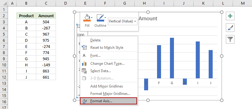
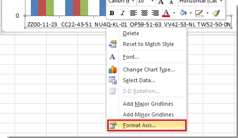
How to Create Venn Diagram in Excel – Free Template Download Step #9: Change the horizontal and vertical axis scale ranges. Rescale the axes to start at 0 and end at 100 to center the data markers near the middle of the chart area. Right-click on the vertical axis and select “Format Axis.” In the Format Axis task pane, do the following: Navigate to the Axis Options tab. Set the Minimum Bounds to “0.”

How to move chart X axis below negative values/zero/bottom in Excel?

Add filter option for all your columns in a pivot table - Excel Exercise If you select the cell locate next to the header column of your pivot table. In this situation, the menu Data > Filter is enabled. And then, all your pivot table columns have the filter options. With all the features related to filters. Select of specific values.

30 How To Label A Cell In Excel - Labels Database 2020

boxplot() in R: How to Make BoxPlots in RStudio [Examples] library (dplyr) library (ggplot2) # Step 1 data_air <- airquality % > % #Step 2 select (-c (Solar.R, Temp)) % > % #Step 3 mutate (Month = factor (Month, order = TRUE, labels = c ("May", "June", "July", "August", "September")), #Step 4 day_cat = factor (ifelse (Day < 10, "Begin", ifelse (Day < 20, "Middle", "End"))))

Advanced Graphs Using Excel : 3D-histogram in Excel

Data Visualization 101: How to Choose the Right Chart or Graph for Your ... Start the y-axis at 0 to appropriately reflect the values in your graph. 2. Bar Graph. A bar graph, basically a horizontal column chart, should be used to avoid clutter when one data label is long or if you have more than 10 items to compare. This type of visualization can also be used to display negative numbers.

How to rotate axis labels in chart in Excel?

Fill Blank Cells in Excel Column - Contextures Excel Tips The first main step is to select all the blank cells that you want to fill. To select the empty cells with Excel's built in Go To Special feature, follow these steps: Select columns A and B, that contain the blank cells. Use the Ribbon commands: On the Excel Ribbon's Home tab, in the Editing group, click Find & Select.

Dynamic Chart Titles in Excel | EngineerExcel

how to plot multiple y axis in excel - firststepimmigration.com Click on the right-hand axis and select format axis, then under the axis option tab, select maximum to set it to be fixed, and set the value to 100 In Axis Options, select the Maximum from Auto to fixed and enter a value 100 manually and close the format axis window 3. You can, however, create that effect with a bit of a workaround.

Changing Axis Labels in PowerPoint 2013 for Windows

Free Microsoft Excel 77-420 Exam Dumps, Microsoft Excel 77 ... - Exam-Labs Study with Exam-Labs 77-420 Excel 2013 Exam Practice Test Questions and Answers Online. How it works ... Horizontal Axis Labels: "IDs" column in table Series 1: "Zero Scores" column in table. ... Change the text by typing to: Math 1080 - Section 3 Assignments. Show correct answer. Question #30.

How To Change Default Browser In Outlook 2016

Excel Blog - techcommunity.microsoft.com What's New in Excel for the web (March 2022) Avital Nevo on Mar 14 2022 11:31 AM. New conditional formatting experience, function library, filter menu, and more. 7,279.

Raj Excel: Microsoft Excel 2013 Short Cut Keys: Ctrl + Shift + L ...

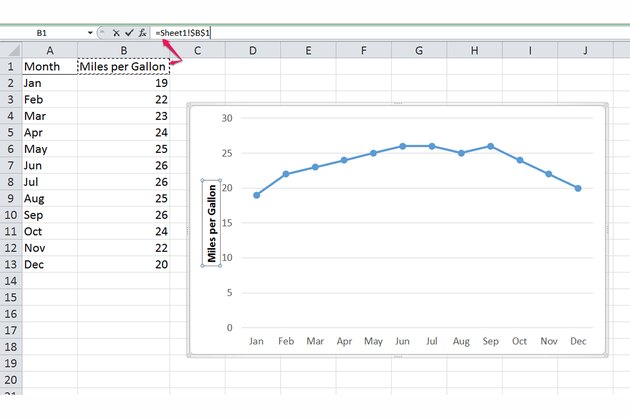
How to Create a Dynamic Chart Title in Excel First of all, just enter the below formula in the formula bar in a new cell. ="Monthly Sales Trend: " &H3 Select the chart title. Go to formula bar and press =. Now, just select the new cell. Hit enter. Creating Dynamic Title in Pivot Chart You can also use the same method to create a dynamic title in a pivot chart.

Share :